
If the net present value of an investment is inversely related to the discount rate, there must be a specific discount rate at which the NPV becomes zero. This discount rate is known as the internal rate of return (IRR) or yield to maturity. In the context of capital investment, you can use “IRR” instead of “yield to maturity” since both terms refer to the same concept—yield to maturity pertains to financial securities, while IRR is used in the context of capital expenditures.
1. HOW IS IT DETERMINED?
To calculate IRR, you just have to make “r” the unknown and simply use the NPV formula again. The rate r is determined as follows:
\[NPV = \sum_{n=1}^{N}\frac{F_n}{(1+r)^n}-V_0\]Put simply, the internal rate of return of an investment is the rate at which its market value equals the present value of its future cash flows. One way to find the IRR is through trial and error. This involves identifying an interest rate that produces a negative net present value and another that results in a positive net present value. These values create a range that can be progressively narrowed down until the yield to maturity is determined.
Clearly, this method can be quite time-consuming. It’s much more efficient to use a calculator or a spreadsheet program with a built-in function to calculate the yield to maturity.
2. THE USE AS AN INVESTMENT CRITERION
The internal rate of return is commonly used in financial markets because it provides investors with an immediate indication of the expected return relative to a specific level of risk. Investors can then compare this expected return to their required return rate, making the investment decision process more straightforward.
The decision-making rule is simple: if an investment’s IRR exceeds the investor’s required return, the investment or security should be pursued. If the IRR is lower, the investment should be avoided or the security sold. An investment is considered worthwhile when its IRR is equal to or greater than the investor’s required return. Conversely, if the IRR is below the required return, the investment should not be made.
At fair value, the internal rate of return matches the market return, meaning the net present value is zero.
3. THE LIMITS
With this new criterion for making investment decisions, it’s important to explore how the internal rate of return interacts with net present value. Additionally, it’s worth examining whether these two criteria might ever lead to conflicting conclusions. When it comes to deciding whether to invest in a particular project or security, both criteria yield the same outcome, as demonstrated in the example. If the cash flow schedule remains consistent, calculating the NPV using a selected discount rate and determining the IRR (and comparing it to the discount rate) are essentially two perspectives on the same mathematical concept.
However, the situation becomes more nuanced when selecting between multiple projects or securities, which is often the case. Comparing different streams of cash flows (securities) is necessary to make an informed choice between them.
The modified IRR
Let’s consider two investments, A and B, with the following cash-flows:
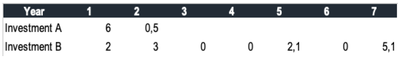
At a 5% discount rate, the present value of investment A is 6.17, and the present value of investment B is 9.90. With a market value of 5 for investment A, its net present value is 1.17. For investment B, with a market value of 7.5, the NPV is 2.40. The internal rate of return is 27.8% for investment A and 12.7% for investment B. To summarize:
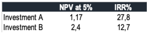
Investment A offers a much higher rate of return than required (27.8% vs. 5%) but over a shorter period. Investment B’s return is lower (12.7% vs. 27.8%) but still exceeds the required rate and lasts longer (seven years vs. two). This creates a conflict between NPV and IRR models, making it unclear whether to choose Investment A or B. On the surface, Investment B seems preferable due to its higher NPV and greater value creation (2.40 vs. 1.17). However, Investment A might be seen as better because its cash flows are received sooner, allowing for earlier reinvestment in high-return projects. Yet, exceptional returns are unlikely to be sustained, as competition and arbitrage usually drive NPVs toward zero and return rates toward the required rate.
Given this, it’s more realistic to assume that Investment A’s cash flows will be reinvested at the required rate of return (5%). This aligns with the NPV approach, which assumes reinvestment at the required rate, unlike the IRR, which assumes reinvestment at the IRR rate—an assumption that is often unrealistic.
The Modified IRR (MIRR) addresses this issue by calculating the rate of return that results in an NPV of zero when comparing the initial investment to the terminal value of the project’s net cash flows, reinvested at the required rate of return.
Determining the Modified IRR involves two steps:
- Calculate the terminal value of the project by compounding all intermediate cash flows to the end of the project at the required rate of return.
- Determine the internal rate of return that equates this terminal value with the initial investment.
For investments A and B, we capitalize their cash flows at the required rate of return (5%) up to period 7.
For Investment A, this results in a terminal value of 6×1.056+0.5×1.055=8.68
For Investment B, the terminal value is 2×1.056+3×1.055+2.1×1.052+5.1=13.9
The MIRR is 8.20% for Investment A and 9.24% for Investment B.
This reconciles the NPV and IRR models. Some might argue that it’s inconsistent to expect Investment A to be more valuable than Investment B since only 5 was invested in A versus 7.5 in B. Even if we were to invest an additional amount to equalize the purchase price, the adjusted NPV for Investment A would be 1.76, still lower than Investment B’s NPV of 2.40. Given the high return of Investment A, it’s unlikely to find another investment with the same return.
Instead, we should assume that any additional investment would yield the required return of 5% over seven years. In this case, the NPV would remain 1.17, but the MIRR would drop to 11%. Consequently, NPV and MIRR would both suggest that Investment B is the more attractive option.
IV. YIELD TO MATURITY
After examining the yield to maturity, you have to consider interest rates, such as those associated with a loan you might take out. Where does the interest rate fit into this context? Suppose someone offers to lend you €1,000 today at an interest rate of 10% for five years. This 10% represents the annual nominal interest rate for the loan and will be used to calculate interest based on the elapsed time and the amount borrowed. Assume interest is paid annually.
The next consideration is how and when you will repay the loan. Repayment terms define the method of loan amortization. For example:
Bullet repayment
The entire loan is paid back at maturity:
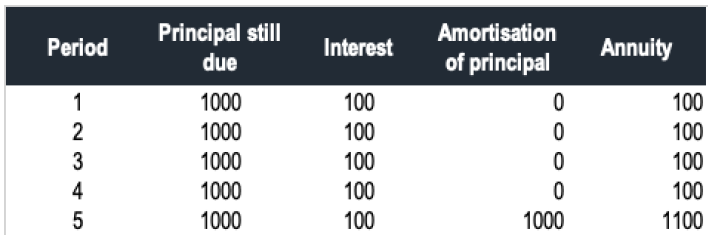
Total debt service refers to the annual amount that includes both interest and principal repayments. This is also known as debt servicing for each payment period.
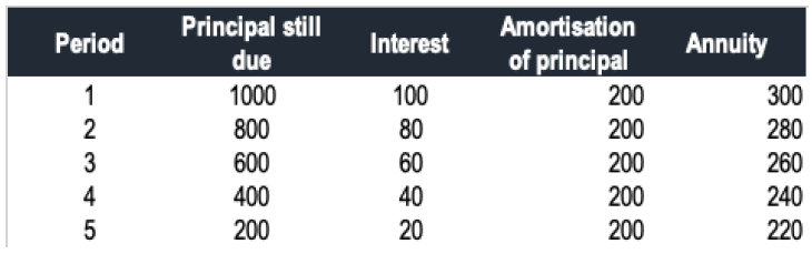
Constant amortization
Each year, the borrower repays a fixed fraction of the principal, calculated as 1/n, where n represents the original term of the loan. The cash flow table would appear as follows:
Understanding Effective Annual Rate
When interest is paid multiple times a year, it impacts the overall cost or return of a loan. For example, if you borrow money at a nominal rate of 10%, but interest is paid semi-annually, the situation differs from paying all interest once a year. In the semi-annual case, you might pay interest twice a year, which you could have kept and invested if it were an annual payment.
The effective annual rate (EAR) helps compare loans with different payment schedules. If interest compounds more frequently, such as every six months, the effective rate is higher than the nominal rate due to interest compounding on itself. For a 10% nominal rate with semi-annual payments, the effective rate becomes higher because interest is calculated on interest more frequently.
To accurately compare investments or loans with varying payment schedules, the EAR should be calculated. This ensures that different cash flow streams are assessed on a consistent annual basis, making meaningful comparisons possible, unlike nominal rates which can be misleading.