To estimate the risk premium in a fairly valued market, it’s essential to ask: What premium should be added to the risk-free rate to determine the required rate of return? Investors should start with the market portfolio and then adjust their exposure by borrowing or investing in risk-free assets based on their risk tolerance. This approach helps in evaluating an investment by considering the additional risk and return it contributes to the market portfolio.

Investment risk is often broken down into components, specifically the security’s volatility and the market’s overall volatility. The objective is to transition from r (the discount rate used in company valuation) to k (the return investors expect on a specific security). This method assumes the investor has a diversified portfolio. While higher risk demands a higher return, a single investment’s failure can negate the benefits, which underscores the importance of diversification. The relevance of the risk premium emerges when it’s spread across multiple investments, making portfolio management and diversification vital in finance.

Unlike a financial investor, an entrepreneur with a single investment must minimize risk through effective management, as they lack the cushion of diversification. In contrast, financial investors rely on portfolio management to assess the risk and return of each investment, applying basic portfolio theory to make informed decisions.

1. THE RETURN REQUIRED BY INVESTORS

The Capital Asset Pricing Model (CAPM), developed in the late 1950s and 1960s by Harry Markowitz, William Sharpe, John Lintner, and Jack Treynor, has become a universally applied financial model. CAPM assumes that investors act rationally, using all relevant information on financial securities to maximize returns at a given level of risk, as discussed in earlier chapters on efficient markets and investor behavior.
While the capital market line describes the return of a portfolio, CAPM focuses on determining the required return for a specific security based on its risk. To minimize total risk, investors diversify their portfolios, thereby reducing specific, or diversifiable, risk. As a result, when stocks are fairly valued, investors are compensated only for the portion of risk they cannot eliminate—the market, or non-diversifiable, risk. In a market where arbitrage is possible, investors won’t receive additional compensation for risks they can mitigate through diversification.

The key insight from portfolio theory is that an investor’s required rate of return is tied solely to market risk, not total risk. In a fairly valued market, diversifiable risk isn’t rewarded. Therefore, the required rate of return (k) is equal to the risk-free rate (rF) plus the risk premium for non-diversifiable, or market, risk, as expressed in the CAPM formula:

Or:

The required rate of return for the market (Km) and the sensitivity coefficient (β) are key components of the CAPM formula. The risk-free rate (Rf) is the return on a risk-free asset, which equals the actual return received since there’s no risk involved. It’s important to note that the β coefficient measures an asset’s non-diversifiable risk, not its total risk. Therefore, a stock might be generally risky but have a low β if it’s weakly correlated with the market.

The difference between the expected return on the market and the risk-free rate is known as the equity risk premium. In developed economies, this typically ranges from 3% to 6%, but it’s higher in emerging markets. For instance, during the 2008 financial crisis, the equity risk premium soared to around 10% before gradually declining to about 6% by 2014.

There are two types of equity risk premiums: historical and expected. The historical risk premium is calculated as the annual return of equity markets (including dividends) minus the risk-free rate. The expected risk premium, which is used in CAPM, isn’t directly observable but can be estimated by forecasting future cash flows of all companies, calculating the discount rate that equates those cash flows with current share prices, and then subtracting the risk-free rate.

To determine the risk premium for an individual stock, multiply the market risk premium by the stock’s beta coefficient. For example, if the risk-free rate is 3.15% and the expected risk premium is 6.25%, a shareholder in Lufthansa, with a β of 1.31, would expect a return of 3.15% + 1.31 × 6.25% = 11.34%. Meanwhile, a shareholder in Tesco, with a β of 0.83, would expect a return of 3.15% + 0.83 × 6.25% = 8.34%. This illustrates how different β values influence expected returns based on market risk.

2. THE PROPERTIES OF CAPM

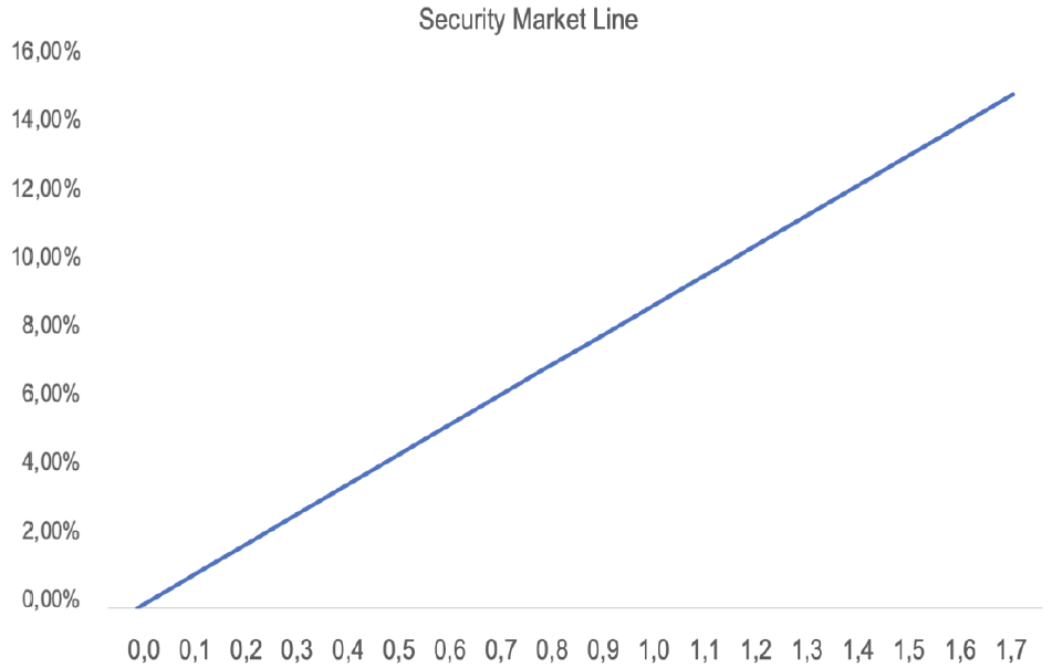
Security market line

The security market line is plotting expected returns on the y-axis against each stock’s beta coefficient on the x-axis. It’s a valuable tool for determining the required rate of return on a security based on the only risk that is compensated—the market risk.

Changes in the market can be understood by observing shifts in this line:

• A parallel shift with no change in slope (i.e., no change in the risk premium) reflects market changes due to interest rate fluctuations. For instance, a drop in interest rates usually causes a downward shift, leading to a general increase in stock prices.
• A non-parallel shift (or pivot) indicates a change in the risk premium, affecting the compensation for risk. In this scenario, riskier stocks will experience greater movement, while less risky stocks may remain relatively stable.

The position of individual stocks relative to the securities market line also serves as a decision-making tool. If a stock, like Prada, is above the line, it offers a higher expected return for its risk, suggesting it’s undervalued. Investors might buy it, driving up the price and lowering the expected return. Conversely, a stock below the line, like Boeing, is considered overvalued. However, it’s important to act with caution, as stock prices may have already adjusted by the time you review such charts.

3. THE LIMITS OF CAPM

The Capital Asset Pricing Model (CAPM) is widely used in modern finance, based on the assumption that markets are efficient. However, there are several practical issues with the model that critics often highlight.

Limits of Diversification

CAPM builds on portfolio theory, which assumes that diversification helps reduce non-diversifiable risk. Research shows that achieving effective diversification has become more complex over time. In the 1970s, a portfolio of 20 stocks could significantly reduce risk, but today at least 50 stocks
are needed to achieve the same effect. This complexity arises from increased volatility of individual stocks, the rise of riskier sectors like biotechnology and technology, and the decline of diversified conglomerates. Additionally, the correlation between market returns and individual stocks is decreasing, which may weaken CAPM’s relevance as the significance of β diminishes.

The forecast beta

A major criticism of beta is its instability over time. While beta condenses extensive information into a single figure, this very simplicity can be a drawback. CAPM, used for forecasting, relies on beta to estimate expected returns based on anticipated risk. Given that beta can fluctuate, it is often more effective to use a forecasted β rather than a historical value.

To address this, calculations should account for earnings and dividend consistency and sector visibility. Research has suggested that beta tends to converge towards 1, but this is counterintuitive since some sectors consistently exhibit a beta above 1. Additionally, recent economic crises have shown that the disparity between high and low beta values tends to widen during challenging periods.

The theoretical limits of CAPM

The CAPM operates under the assumption that markets are fairly valued. However, markets are not always at fair value, as evidenced by the popularity of technical analysis, which indicates doubts about market efficiency. The CAPM also assumes that market participants have rational expectations and that the model is universally accepted as correct. The development of alternative theories suggests that this universal acceptance is not guaranteed.

Consequently, it is viewed as just one theoretical framework for financial markets. Although other theories and methods exist, they have not yet matched the CAPM’s appeal due to its straightforward concepts. Nonetheless, there is optimism that some criticisms of the CAPM might be resolved. For instance, research suggests that the model’s shortcomings could stem from an inaccurate estimation of the market portfolio and might be addressed by including not just stocks but also bonds and other investments, as the theory originally intended.

4. MULTIFACTOR MODELS

Arbitrage Pricing Theory (APT)

The APT model extends the CAPM by considering multiple factors affecting security returns, rather than relying solely on market risk. Proposed by Stephen Ross, APT includes various macroeconomic variables and company-specific factors. For a given security J, the return is calculated as:

Unlike the CAPM’s single-factor approach, APT does not specify which macroeconomic variables to use; Ross’s original study included factors such as inflation, manufacturing output, risk premium, and the yield curve. This model replaces the challenging measurement of market return with multiple variables but is more suited for portfolio management rather than stock valuation.

Fama–French model

The Fama–French model, an extension of APT, focuses on company-specific factors to explain historical returns. Developed by Eugene Fama and Kenneth French, it incorporates three key factors: market return, price-to-book value ratio, and the return gap between large and small-cap stocks, which suggests a liquidity effect. The model can also include additional factors like P/E ratio, market capitalization, and past performance, challenging the efficient market theory.

Liquidity premium, size premium, and investor protection

Liquidity and its impact on returns are significant factors in determining risk. Some research shows a liquidity premium for small-cap stocks, while large-cap stocks do not exhibit this premium. In their model, the expected return on a security includes both the market premium and the liquidity premium. This approach, which adds the liquidity premium to the CAPM-derived return, contrasts with the “liquidity discount” concept.

While the CAPM is foundational, its limitations underscore the need for more comprehensive models. Alternatives like APT and the Fama–French model, along with liquidity considerations, offer valuable insights, and integrating these approaches could enhance investment evaluations in evolving markets.